Introduction of RL
Math
主要介绍需要用到的概率论的基础知识以及强化学习中关键术语。
Random Variable
通常使用大写字母(如:X)表示随机变量, 使用小写字母(如:x, x1)表示随机变量的观测值(observed value),观测值是确定的数,没有随机性。
Probability Density Function(PDF)
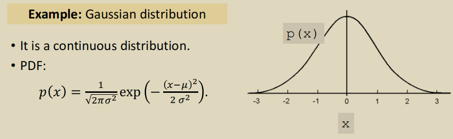
概率密度函数:PDF provides a relative likelihood that the value of the random variable would equal that sample.
例如:连续的正态分布(也叫做高斯分布)
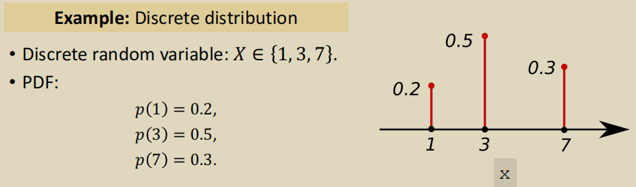
离散的分布:
假设随机变量 X 的域为 \(\mathbb{X}\)
连续分布
\(\int_\mathbb{X} p(x)dx = 1\)
期望: \(\mathbb{E}[f(x)] = \int_{x\in \mathbb{X}}{p(x) \cdot f(x)}dx\)
离散分布
\(\sum_{x \in \mathbb{X}}{p(x)} = 1\)
期望:\(\mathbb{E}[f(x)] = \sum_{x\in \mathbb{X}}{p(x) \cdot f(x)}\)
Random Sampling
随机采样:1. 知道各情况种类以及总数,去抽样 2. 知道各情况概率,去抽样。
Terminology
state and action
policy
Policy function \(\pi\) 是动作 A 的概率密度函数: \(\pi(a|s) = P(A=a|S=s)\) 它是在某状态 s 下,采取某个特定动作(例如:A=a1)的概率。 例如:给定状态 s,动作 A 离散分布的概率密度函数如下:
- \(\pi(left|s) = 0.2\)
- \(\pi(right|s) = 0.2\)
- \(\pi(up|s) = 0.2\)
- \(\pi(down|s) = 0.2\) 根据选取的策略不同(随机性策略或者确定性策略),从中随机选取或者选取概率最大的 action 进行实施。
reward
state transition
\(old state \xrightarrow{action} new state\)
- State transation can be random
- Randomness is from the environment(状态转移的随机性取决于环境,这里的环境就是游戏程序)
- 状态转移,用 p 函数表示: \(p(s^{'}|s,a) = \mathbb{P}(s^{'}=s,A=a)\), 如果观察到当前状态 s 和动作 a,P 函数输出状态变为 \(p(s^{'}\) 的概率。
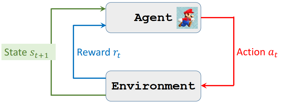
agent environment interaction
Randomness in Reinforcement learning
Actions have randomness
Given state 𝑠, the action can be random
State transitions have randomness
Given state 𝑆 = 𝑠 and action 𝐴 = 𝑎, the environment randomly generates a new state \(𝑆^{'}\)
Rewards and Returns
Return
Definition: Return (aka cumulative future reward) \(𝑈_{t} = 𝑅_{t} + 𝑅_{t+1} + 𝑅_{t+2} + 𝑅_{t+3} + ⋯\)
- Future reward is less valuable than present reward.
- \(R_{t+1}\) should be given less weight than \(𝑅_{t}\)
Discounted return
Definition: Discounted return (aka cumulative discounted future reward)
- \(\gamma\): discount rate (tuning hyper-parameter)
- \(𝑈_{t} = 𝑅_{t} + \gamma𝑅*{t+1} + \gamma^2𝑅*{t+2} + \gamma^3𝑅_{t+3} + ⋯\)
At time step 𝑡, the return \(𝑈_{t}\) is random. Two sources of randomness:
- Action can be random: \(ℙ[𝐴=𝑎|𝑆=𝑠]=𝜋(𝑎|𝑠)\)
- New state can be random: \(ℙ[𝑆^{'}=𝑠^{'}|𝑆=𝑠,𝐴=𝑎]=𝑝(𝑠^{'}|𝑠,𝑎)\)
- For any 𝑖 ≥ 𝑡, the reward 𝑅n depends on 𝑆n and 𝐴n.
- Thus, given 𝑠, the return 𝑈 depends on the random variables:
- \(𝐴_{t},𝐴_{t+1},𝐴_{t+2},⋯\) and \(𝑆_{t+1},𝑆_{t+2},⋯\)
Action-Value Function 𝑄(s,a)
Definition: Action-value function for policy 𝜋
\(𝑄_{\pi}(𝑠_{t},𝑎_{t}) = \mathbb{E}[𝑈_{t}|𝑆_{t}=𝑠_{t}, 𝐴_{t}=𝑎_{t}]\)
- Return \(𝑈_{t}\) depends on states \(𝑆_{t},𝑆_{t+1},S_{t+2},⋯\) and actions \(A_{t},A_{t+1},A_{t+2},⋯\)
- 将随机变量 \(𝑈_{t}\) 当作未来所有状态 S 以及未来所有动作 A 的一个函数求期望,将这些变量积分积掉,得到一个数 \(𝑄_{\pi}\)。
- \(𝑆_{t}, A_{t}\) 被作为观测到的数值而对待,没有被积掉了。因此 \(𝑄_{\pi}\) 的值与 \(𝑆_{t}, A_{t}\) 有关。
- 积分的时候会用到 Policy 函数,如果 Policy 函数 \(\pi\) 不一样,积分得到的函数 \(𝑄_{\pi}\) 就不一样。
未来状态和动作都有随机性
- Actions are random: \(\mathbb{P}[A=a|S=s]=\pi(a|s)\), 动作 A 的概率密度函数是 Policy function \(\pi\)
- States are random: \(\mathbb{P}[S^{'}=s^{'}|A=a]=p(s^{'}|s,a)\), 状态 S 的概率密度函数是 state transition function p.
\(𝑄_{\pi}\) 的意义:采取策略 \(\pi\),在 \(S_{t}\) 状态下,动作 \(A_{t}\) 的好坏。
Optimal action-value function
用不同的策略 \(\pi\), 就有不同的 \(𝑄_{\pi}\), 那如何将 Action-Value function 中的 \(\pi\) 去掉呢?答案是: \(𝑄_{\pi}\) 关于 \(\pi\) 求最大化。
Definition: Optimal action-value function.
\(Q^{\star}\left(s_{t}, a_{t}\right)=\underset{\pi}{\max} Q_{\pi}\left(s_{t}, a_{t}\right)\)
使用最好的策略 \(\pi\)(也就是使得 \(𝑄_{\pi}\) 函数最大化的那个 \(\pi\)),因此 \(Q^{\star}\) 与 \(\pi\) 无关了,它只与 \(S_{t}, A_{t}\) 有关。
\(Q^{\star}\) 的意义:在某个状态 s 下,对动作 a 做评价。
State-value function
- \(V_{\pi}(s_{t}) = \mathbb{E_{A}}[Q_{\pi}(s_{t}, A)] = \sum{\pi(a|s_{t})\cdot Q_{\pi}(s_{t},a)}\) (Actions are discrete)
- \(V_{\pi}(s_{t}) = \mathbb{E_{A}}[Q_{\pi}(s_{t}, A)] = \int{\pi(a|s_{t})\cdot Q_{\pi}(s_{t},a)}da\) (Actions are continuous)
将动作 A 当作随机变量,对其进行积分求期望, 其中 A 的概率密度函数 \(A~\pi(\cdot|s_{t})\),将 A 消掉,然后 \(V_{\pi}\) 函数就只与 \(\pi\) 和 S 有关。
意义:\(V_{\pi}\) 可以告诉我们当前的局势状况好坏优劣。
Value Functions
Action-value function
\(𝑄_{\pi}(𝑠_{t},𝑎_{t}) = \mathbb{E}[𝑈_{t}|𝑆_{t}=𝑠_{t}, 𝐴_{t}=𝑎_{t}]\)
For policy \(\pi\), \(𝑄_{\pi}(𝑠_{t},𝑎_{t})\) evaluates how good it is for an agent to pick action a while being in state s.
State value function
\(V_{\pi}(s*{t}) = \mathbb{E_{A}}[Q_{\pi}(s_{t}, A)] = \sum_{a} \pi\left(a \mid s_{t}\right) \cdot Q_{\pi}\left(s_{t}, a\right)\)
如果动作 A 的概率密度函数 \(\pi\) 是离散的,则 \(V_{\pi}\) 可以进一步写成求和的形式;如果是连续的,则可写为积分形式。
For fixed policy \(\pi\), \(V_{\pi}(s_{t})\) evaluates how good the situation is in state s.
\(\mathbb{E}_{s}[V_{\pi}(S)]\) evaluates how good the policy \(\pi\) is.
Two Methods
Policy-based:Suppose we have a good policy \(\pi(a|s)\).
- Upon observing the state \(S_{t}\)
- random sampling \(a_{t}~\pi(\cdot|s_{t})\)
Value-based:Suppose we know the optimal action-value function \(Q^{\star}(s|a)\)
- Upon observe the state \(S_{t}\)
- choose the action that maximizes the value \(a_{t} = argmax_{a}Q^{\star}(s_{t},a)\)
几种分类
| 通过价值选行为 | 直接选行为 | 想象环境并从中学习 |
|---|---|---|
| Q learing | Policy Gradient | Model based Rl |
| Sarsa | ||
| Deep Q Network |
理解环境
根据理解环境与否, 分为 Model-Free RL 与 Model-Based RL
Model-Free
特点:不尝试理解环境,根据环境的反馈一步步学习 代表:Q Learning、Sarsa、Policy Gradients
Mode-Based
特点:建模,可以自己训练
概率与价值
基于概率(Policy-Based RL)、基于价值(Value-Based RL)
基于概率(Policy-Based RL)
根据所处的环境,判断下一步行动的概率,每一种动作都有可能被选中,只是可能性大小不同 使用连续的概率分布处理选择连续的动作 代表:Policy Gradients
基于价值(Value-Based RL)
直接选择价值最高的动作;无法处理连续的动作 代表:Q Learning、Sarsa
结合 Policy 和 Value 的 Actor-Critic
Actor: 基于概率做出动作 Critic: 根据做出的动作给出价值
更新频率
回合更新(Monte-Carlo update) 等待每次训练结束,进行更新 代表:基础版 Policy Gradients、Monte-Carlo Learing
单步更新(Temporal-Difference update) 训练过程中的每一步都进行更新 代表:Q Learning、Sarsa、升级版 Policy Gradients
在线与离线
在线学习 本人在场,边玩边学习 代表:Sarsa、Sarsa(Lambda)
离线学习 可以从他人的经历中进行学习 也可以白天存储学习经验,晚上离线学习 代表:Q Learning、Deep Q Network
Going to learn
Value-based learning.
- Deep Q network (DQN) for approximating \(𝑄^{\star}(𝑠|𝑎)\).
- Learn the network parameters using temporal different(TD).
Policy-based learning.
- Policy network for approximating 𝜋(𝑎|𝑠).
- Learn the network parameters using policy gradient.
Actor-critic method. (Policy network + value network.)
Example: AlphaGo
资料
- 2015 年 David Silver 的经典课程Teaching
- 2017 年加州大学伯克利分校 Levine, Finn, Schulman 的课程 CS 294 Deep Reinforcement Learning, Spring 2017
- 卡内基梅隆大学的 2017 春季课程Deep RL and Control。