从 LeNet5 学 CNN

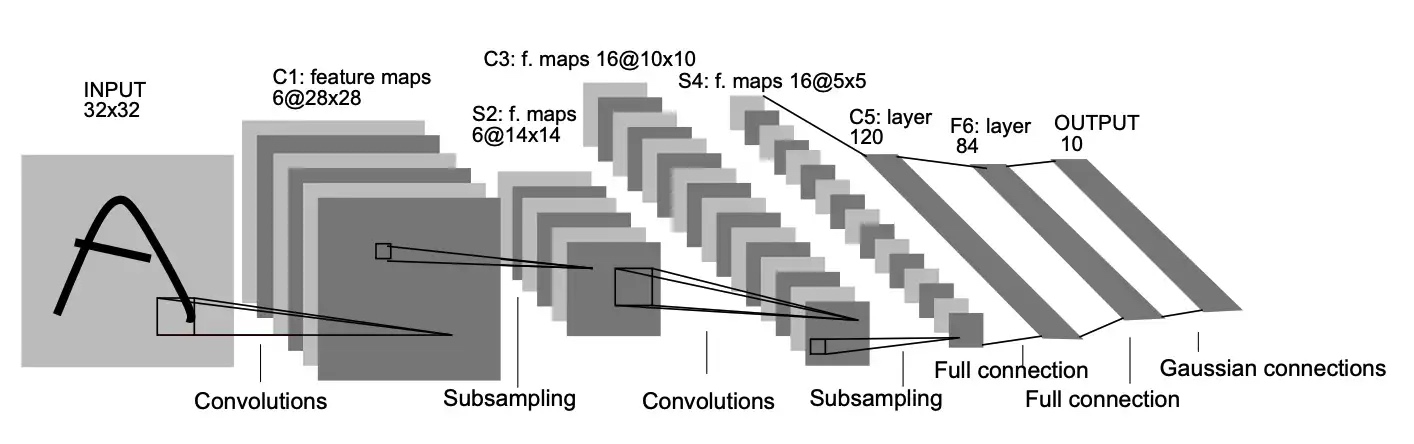
LeNet-5 comprises seven layers, not counting the input, all of which contain trainable parameters (weights). The input is a 32x32 pixel grayscale image.

16696231411578 The naming convention used by the authors:

Cx — convolution layer,
Sx — subsampling (pooling) layer,
Fx — fully-connected layer,
x — index of the layer.

The formula for calculating the output size of the convolutional layer.

\[(W−F+2P)/S+1\]

, where W is the input height/width (normally the images are squares, so there is no need to differentiate the two), F is the filter/kernel size, P is the padding, and S is the stride.

Description of the LeNet-5 architecture layer by layer.

Layer 1 (C1): convolutional layer

Input: 1x32x32 pixel (in_channel=1 means that the grayscle image only have one channel)

Process: 6 kernels/filters/feature maps of size 5x5 and the stride is 1 If in_channel=3. means that the image have 3 channels, like RGB image. The kernel will extract 3 channels, that is, for each channel, there are 6 kernels of size 5x5, which is 6x3 tensors of 5x5

Ouput: 1x28x28x6 According to the formula: (32-5+2*0)/1+1=28, and each kernel will extracts a channel.
Layer 2 (S2): subsampling/pooling layer

The subsampling layer in the original architecture was a bit more complex than the traditionally used max/average pooling layers. I will quote [1]: “ The four inputs to a unit in S2 are added, then multiplied by a trainable coefficient, and added to a trainable bias. The result is passed through a sigmoidal function.”. As a result of non-overlapping receptive fields, the input to this layer is halved in size (14×14×6).】

Input: 28x28x6 Proccess: avg or max pooling layer, the stride is 2 Output： 14x14x6
Layer 3 (C3): The second convolutional layer with the same configuration as the first one, however, this time with 16 filters. The output of this layer is 10×10×16.
Layer 4 (S4): The second pooling layer. The logic is identical to the previous one, but this time the layer has 16 filters. The output of this layer is of size 5×5×16.

Ouput: 5×5×16 池化层是当前卷积神经网络中常用组件之一，它最早见于 LeNet 一文，称之为 Subsample。自 AlexNet 之后采用 Pooling 命名。池化层是模仿人的视觉系统对数据进行降维，用更高层次的特征表示图像。

实施池化的目的：(1) 降低信息冗余；(2) 提升模型的尺度不变性、旋转不变性；(3) 防止过拟合。池化层的常见操作包含以下几种：最大值池化，均值池化，随机池化，中值池化，组合池化等。

池化的超级参数包括过滤器大小和步幅，常用的参数值为，，应用频率非常高，其效果相当于高度和宽度缩减一半。最大池化时，往往很少用到超参数 padding，最常用的值是 0

最大池化只是计算神经网络某一层的静态属性，池化过程中没有需要学习的参数。执行反向传播时，反向传播没有参数适用于最大池化。
Layer 5 (C5): The last convolutional layer with 120 5×5 kernels. Given that the input to this layer is of size 5×5×16 and the kernels are of size 5×5, the output is 1×1×120. As a result, layers S4 and C5 are fully-connected. That is also why in some implementations of LeNet-5 actually use a fully-connected layer instead of the convolutional one as the 5th layer. The reason for keeping this layer as a convolutional one is the fact that if the input to the network is larger than the one used in [1] (the initial input, 32×32 in this case), this layer will not be a fully-connected one, as the output of each kernel will not be 1×1.

Input: 5x5x16 Proccess: 120 kernels of size 5x5 Output: 1x1x120

在这里还需要注意的是 C5 层，它是一个比较特殊的卷积层，它的输入是 16 通道 5*5 大小的特征图像，而输出是一个 120 的向量。C5 层可以有两种实现，第一种是使用 5*5 大小的卷积核进行卷积，第二种是将 16 通道 5*5 大小的特征图像拉平，然后再做全连接。
Layer 6 (F6): The first fully-connected layer, which takes the input of 120 units and returns 84 units. In the original paper, the authors used a custom activation function — a variant of the tanh activation function. For a thorough explanation, please refer to Appendix A in [1].

那么全连接层对模型影响参数就是三个：
```
全接解层的总层数（长度）
单个全连接层的神经元数（宽度）
激活函数
首先我们要明白激活函数的作用是：

增加模型的非线性表达能力
```
Layer 7 (F7): The last dense layer, which outputs 10 units. In [1], the authors used Euclidean Radial Basis Function neurons as activation functions for this layer.

Why is the input size of LeNet-5 set to `32x32` when it was initially trained with MNIST using `28x28` images?

The input is a 32x32 pixel image. This is significantly larger than the largest character in the database (at most 20x20 pixels centered in a 28x28 field). The reason is that it is desirable that potential distinctive features such as stroke endpoints or corner can appear in the center of the recep tive field of the highest-level feature detectors

from original paper[2]

code

由于 MNIST 数据集图片尺寸是 28x28 单通道的，而 LeNet-5 网络输入 Input 图片尺寸是 32x32，因此使用 transforms.Resize 将输入图片尺寸调整为 32x32。

LeNet-5 trained with MNIST dataset (PyTorch)

ss

从 LeNet5 学 CNN

Why is the input size of LeNet-5 set to 32x32 when it was initially trained with MNIST using 28x28 images?

code

参考

Why is the input size of LeNet-5 set to `32x32` when it was initially trained with MNIST using `28x28` images?