Probabilities background for Wasserstein Distance
Hypothesis Testing in Probabilities
A statistical hypothesis test is a method of statistical inference used to decide whether the data at hand sufficiently support a particular hypothesis. It including both parametric and non-parametric tests.
Parametric Tesing
Parametric tests are those tests for which we have prior knowledge of the population distribution (i.e, normal), or if not then we can easily approximate it to a normal distribution which is possible with the help of the Central Limit Theorem.
参数检验(parameter test)全称参数假设检验,是指当总体分布已知或可近似(如总体为正态分布)时,根据样本数据对总体分布的统计参数(例如均值、方差等)进行的统计检验。
Nonparametric Testing
Nonparametric tests can and should be broadly defined to include all methodology that does not use a model based on a single parametric family.
非参数检验(Nonparametric tests)与参数检验共同构成统计推断的基本内容。在数据分析过程中,由于种种原因,人们往往无法对总体分布形态作简单假定,此时参数检验不再适用。非参数检验正是一类基于这种考虑,在总体方差未知或知道甚少的情况下,利用样本数据对总体分布形态等进行推断的方法。由于非参数检验方法在推断过程中不涉及有关总体分布的参数,因而得名为“非参数”检验。
常见的非参数检验包括:卡方检验 Chi-Squared Test, Kolmogorov–Smirnov 检验, Wasserstein distance
Terms
To determine the distribution of a discrete random variable we can either provide its Probability mass function (PMF) or cumulative distribution function (CDF).
Probability mass function, PMF
A probability mass function (pmf) is a function over the sample space of a discrete random variable X which gives the probability that X is equal to a certain value. The PMF is one way to describe the distribution of a discrete random variable (PMF cannot be defined for continuous random variables).
cumulative distribution function, CDF
The cumulative distribution function (CDF) of a random variable is another method to describe the distribution of random variables. The advantage of the CDF is that it can be defined for any kind of random variable (discrete, continuous, and mixed).
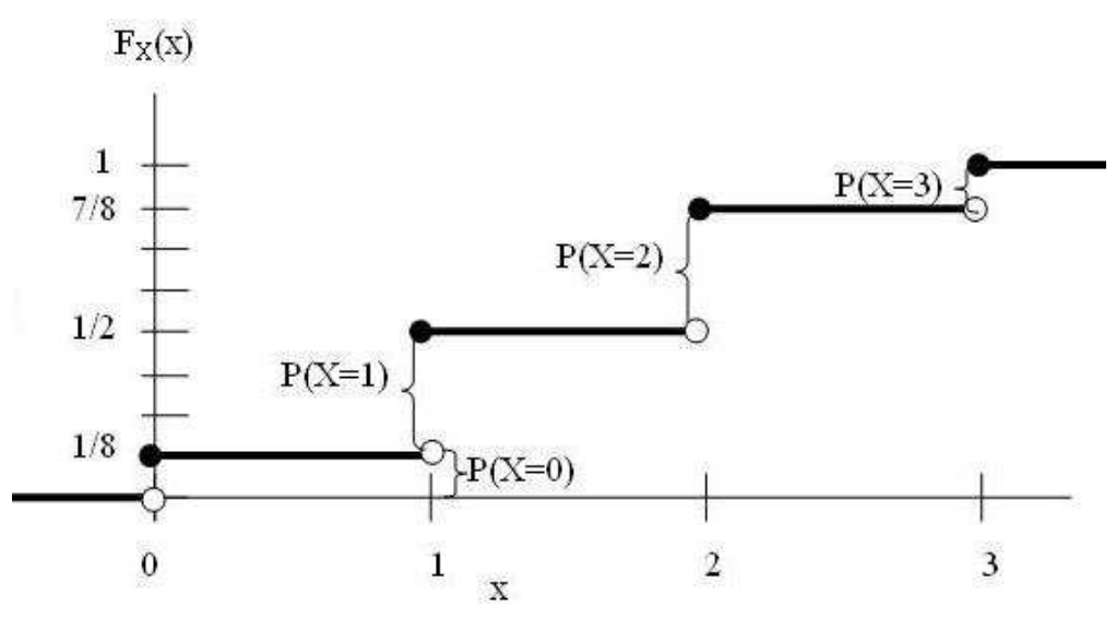
The cumulative distribution function (CDF) of random variable X is the probability that X will take a value less than or equal to \(x\), \(F_X(x)=P(X \le x), \text{for all x} \in \mathcal{R}\).
Probability density function
For continuous random variables, the CDF is well-defined so we can provide the CDF. However, the PMF does not work for continuous random variables, because for a continuous random variable \(P(X = x) = 0, \text{for all x} \in \mathcal{R}\). Instead, we can usually define the probability density function (PDF). The PDF is the density of probability rather than the probability mass.
Quantile function (inverse CDF)
Since the cdf \(F\) is a monotonically increasing function, it has an inverse; let us denote this by \(F^{−1}\). If 𝐹 is the cdf of 𝑋, then \(F^{−1}(\alpha)\) is the value of \(x_a\) such that \(P(X \le X_a) = \alpha\); this is called the \(\alpha\) quantile of \(F\)
The cumulative distribution function takes as input 𝑥 and returns values from the [0,1] interval (probabilities)—let's denote them as 𝑝. The inverse of the cumulative distribution function (or quantile function) tells you what \(x\) would make \(F(x)\) return some value 𝑝, \(𝐹^{−1}(𝑝) = x\)
Joint probability distribution
With the Joint probability distribution, we can conclude the marginal distributions. However, according two marginal distributions \(P\) and \(Q\), the joint distribution is not unique, whose space can be denoted as \(\prod(P_r, P_g)\).
Joint cumulative distribution function is for discrete random variable.
Empirical CDF
Empirical distribution function (commonly also called an empirical cumulative distribution function, eCDF) is the distribution function associated with the empirical measure of a sample. It is an estimator of the Cumulative Distribution Function. The cumulative distribution function is a step function that jumps up by \(\frac{1}{n}\) at each of the n data points.
Let \(X\) be a random variable with CDF \(F(x) = P(X \le x)\), and let \(x_1, x_2, \cdots, x_n\) be n i.i.d random varibales sampled from \(X\) (also called observation values). First, we can sort the observation values in ascending order as \(x_1 \le x_2 \le, \cdots, x_n\), where the frequency of \(x_i\) is \(n_i\) (\(n_1 + n_2 ... + n_3 = n\)). Then, the empirical CDF can be defined as:
\[ F_n(x) = \begin{cases} 0, \quad &(x \lt x_1);\\ \frac{n_1+n_2+\cdots+n_k}{n};\quad &(x_k \le x \lt x_{k+1}); \quad (k=1,2,\cdots, r-1)\\ x,\quad &(x_k \ge x_{r}) \end{cases} \]
or just
\[ \begin{equation} F_n(x_t) = \frac{\text{number of elements in the samples} \le x_t}{n} = \frac{1}{n}\sum_{i=1}^n I_{x_i \le x_t}, \end{equation} \]
where \(I(\cdot)\) is the indicator function. A illustration of empirical CDF of an example is shown below:
References and Recommends
- Parametric and Nonparametric: Demystifying the Terms
- lecture1.pdf](https://www.win.tue.nl/~rmcastro/AppStat2013/files/lecture1.pdf)
- Introduction; The empirical distribution function](https://myweb.uiowa.edu/pbreheny/uk/teaching/621/notes/8-23.pdf)
- Statistical hypothesis testing - Wikipedia
- 非参数检验_百度百科
- Empirical distribution function - Wikipedia
- 样本分布函数 - 快懂百科
- TODO: Empirical Distribution: Everything You Need To Know | by Shubham Panchal | Towards Data Science
- distributions - Help me understand the quantile (inverse CDF) function - Cross Validated