Delve into Wasserstein Distance, principles and implementation analysis

Wasserstein distance

To understand Wasserstein distance fully, It's suggested to first recap the related background of probability theory, which can be seen in my another blog Probabilities background for Wasserstein Distance

Wasserstein distance (also called Wasserstein distance,, optimal transport) is a metric that quantifies the difference between two probability distributions, which is originally proposed in IJCV'2020 《The Earth Mover's Distance as a Metric for Image Retrieval》. It is a normalized measure of the minimum cost of turning one distribution into the other, which can be used to measure the distance between two multi-dimensional distributions. The cost is determined by the amount of "mass" that needs to be moved and the distance it needs to be moved.

Definitions

\[ \begin{equation} W\left(\mathbb{P}_r, \mathbb{P}_g\right)=\inf _{\gamma \in \Pi\left(\mathbb{P}_r, \mathbb{P}_g\right)} \mathbb{E}_{(x, y) \sim \gamma}[\|x-y\|] \end{equation} \]

$\prod(\mathbb{P}_r, \mathbb{P}_g)$ is the set of all joint distributions whose marginals are $P_r$ and $P_g$. The objective is find a joint distribution $\gamma \in \prod(\mathbb{P}_r, \mathbb{P}_g)$ to minimizes the expectation of the distance between $x$ and $y$. The distance $||x-y||$ can be defined as any distance metric, such as Euclidean distance, etc. The minimum expection is the Wasserstein distance between $P_r$ and $P_g$.

For Discrete variables, the Wasserstein distance can be defined as:

Let

$$ \[\begin{equation} \begin{aligned} P &=\{(\mathbf{p}_1, w_{p_1}),(\mathbf{p}_2, w_{p_2}),(\mathbf{p}_3, w_{p_3}), \cdots,(\mathbf{p}_M, w_{p_M})\}, \\ Q &=\{(\mathbf{q}_1, w_{q_1}),(\mathbf{q}_2, w_{q_2}),(\mathbf{q}_3, w_{q_3}), \cdots,(\mathbf{q}_N, w_{q_N})\}, \end{aligned} \end{equation}\] $$

where $p_i$ is the $i$-th point in $P$, $w_{p_i}$ is the weight of $p_i$, $q_j$ is the $j$-th point in $Q$, $w_{q_j}$ is the weight of $q_j$. The $d_{ij}$ is the distance between $P_i$ and $q_j$. The Wasserstein distance between $P$ and $Q$ is defined as:

\[ \begin{equation} \begin{aligned} & \min \sum_{i=1}^M \sum_{j=1}^N d_{i j} f_{i j} \\ \text { s.t } & \\ & f_{ij} \ge 0,\quad i=1,2, \cdots, M ; j=1,2, \cdots, N \\ & \sum_{j=1}^N f_{ij} \leq w_{p_i}, i=1,2, \cdots, M \\ & \sum_{i=1}^M f_{ij} \leq w_{q_j}, j=1,2, \cdots, N \\ & \sum_{i=1}^M \sum_{j=1}^N f_{ij}=\min \left\{\sum_{i=1}^M w_{p_i}, \sum_{j=1}^M w_{p_j}\right\} \end{aligned} \end{equation} \]

EMD is proved to be distance (距离定义必须满足三点：正定性，齐次性，三角不等式) in the original paper. Note that the sum of weight of two difference distribution can be unequal.

Two equavalent formulas

The above definitions is all about optimization. In Why the 1-Wasserstein distance is the area between the two marginal CDFs and On Wasserstein Two Sample Testing and Related Families of Nonparametric Tests, Two equavalent formulas of 1-Wasserstein distance is proved, which are more easily to implement.

For quantile function,

\[ \begin{equation} W_1(X, Y)=\int_{[0,1]}\left|F_X^{-1}(u)-F_Y^{-1}(u)\right| du \end{equation} \]

For cumulative ditribution function,

\[ \begin{equation} W_1(u, v) = \int_{-\infty}^{+\infty} |U-V| \end{equation} \]

1-Wasserstein distance is the area between the two marginal empirical CDFs

Three intuitive and typical examples

Computing the distance of point clouds with different distribution

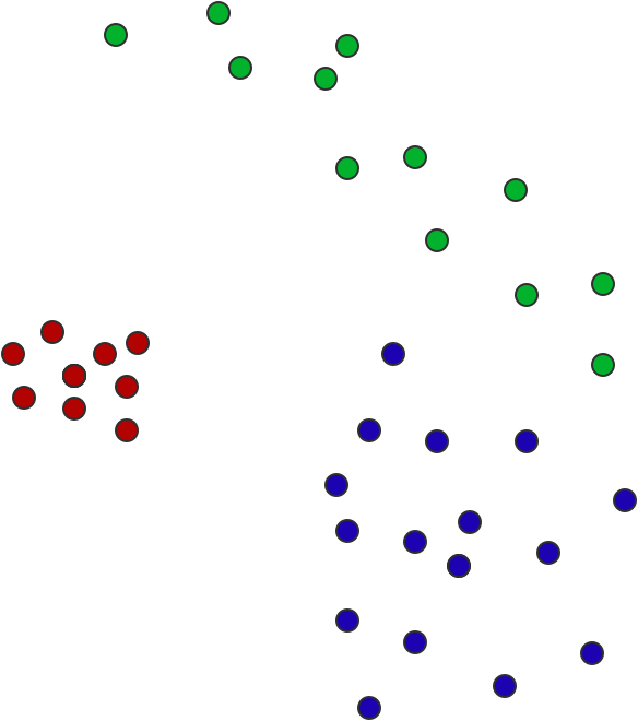
As show in the following figure, there are three point clouds with different distribution, which one is closest to the other two? Blue and red? Red and green? Green and blue?

How to define a distance measure aligning with our intuition about the geometry and distance of the point cloud? The solution is Earth Mover's Distance (EMD)
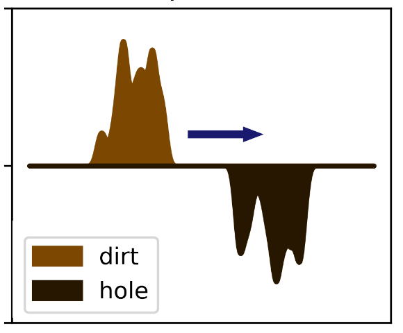
Assume the two probability distribution as dirt and hole, EMD is the cost that needs to be done to move all the dirt to all the holes.

Let us call the above point clouds as sample set A, B, C, which can be regarded as a discrete probability distribution. For each sample $x \in A$, there is $p_x = \frac{1}{|A|}$, where |A| is the total number of points in sample set A. The distance between sample set A and B can be solved by the following linear program:

recall probabilities：a probability mass function (pmf) is a function that gives the probability that a discrete random variable is exactly equal to some value. The probability density function (pdf) is used to describe probabilities for continuous random variables. It's counterpart.

Each $x \in A$ corresponds to a pile of dirt with height $p_x$, and each $y \in B$ corresponds to a hole with depth $p_y$. The cost of moving a unit of dirt from x to y is the Euclidean distance between the two points, denoted as $d(x, y)$. Let $Z_{x,y}$ represent the amount of dirt moved from $x \in A$ to $y \in B$, then the constraints are as follows:
- Each $Z_{x,y} \ge 0$, so dirt can only moves from x to y.
- Every pile $x \in A$ must vanish, i.e. for each fixed $x \in A$, $\sum_{y \in B} Z_{x,y} = p_x$.
- Every hole $y \in B$ must be completely filled, i.e. for each fixed $y \in B$, $\sum_{y \in B} Z_{x,y} = p_x$
The objective is to minimize the cost of moving the dirt, i.e. $\sum_{x,y \in AxB}d(x,y)Z(x,y)$, subject to the linear constraints:

\[ \sum_{x, y \in A \times B}d(x, y)Z_{x,y} \\ s.t \space \{ \begin{split} &Z_{x,y} \ge 0\\ &\sum_{y \in B} Z_{x,y} = p_x\\ &\sum_{x \in A} Z_{x,y} = p_y \\ \end{split} \} \]

Python tools for implementation

Common used tools for Wasserstein distance implementation:

google/or-tools: Google's Operations Research tools:,
scipy, from scipy.stats import wasserstein_distance
POT: Python Optimal Transport — POT Python Optimal Transport 0.9.0 documentation
wmayner/pyemd: Fast EMD for Python: a wrapper for Pele and Werman's C++ implementation of the Earth Mover's Distance metric

An online tools to calculate Wasserstein distance: Monge-Kantorovich Transportation Problem - Wolfram Demonstrations Project

scipy 1d Wasserstein distance

scipy.stats.wasserstein_distance applies to 1D Wasserstein and directly uses L1 norm as the distance metric.

Definitions is the best way to learn: scipy.stats.wasserstein_distance — SciPy v1.11.1 Manual:

scipy.stats.wasserstein_distance(u_values, v_values, u_weights=None， v_weights=None) Compute the first Wasserstein distance between two 1D distributions.

This distance is also known as the earth mover’s distance, since it can be seen as the minimum amount of “work” required to transform $u$ into $v$, where “work” is measured as the amount of distribution weight that must be moved, multiplied by the distance it has to be moved.

u_values, v_values array_like

Values observed in the (empirical) distribution.

u_weights, v_weights array_like, optional

Weight for each value. If unspecified, each value is assigned the same weight. u_weights (resp. v_weights) must have the same length as u_values (resp. v_values). If the weight sum differs from 1, it must still be positive and finite so that the weights can be normalized to sum to 1.

解释：

This function is for Wasserstein-1 distance, where the distance d(x,y) is the L1 norm, absolute value. It's only appliable to 1D distribution, which means 2D distribution should be flatten to 1D.(especially for machine learning weights or images, which is 2D distribution or more)
u_values, v_values are the values observed in the (empirical) distribution, which is the samples drawed from the distribution.

Corresponding to the above example: the position coordinates of the point in the point cloud or the coordinates of dirt and holes.
u_weights, v_weights correspond to the weight of each sample in all samples.

Corresponding to the above example:
1. The weighted number of points at this position in the point cloud (because it is a fraction with weighted sum is 1, so it is called the weighted number)
2. The weighted height, how much, and how deep the dirt and hole are at this position, that is, $p_x$, $p_y$
3. If not specified, the default weights are equal on average. If specified, it needs to be a positive integer and will be normalized to 1
Normally, The way to get wasserstein-1 distance is calculating the distance cost through u_values, v_values, calculate the quality or quantity through u_weights, v_weights, and then establish variables between each point from p to q samples to solve the linear minimum optimization problem.

scipy.stats.wasserstein_distance sourcecode analysis

However, in the scipy function, the wasserstein distance is calculated using the empirical CDFs related definitions in Equation 7

In function scipy.stats.wasserstein_distance, the function _cdf_distance(1, u_values, v_values, u_weights, v_weights) is called with $p=1$ as wasserstein-1 distance.

def _cdf_distance(p, u_values, v_values, u_weights=None, v_weights=None):
    # validate whether it's a distribution
    u_values, u_weights = _validate_distribution(u_values, u_weights)
    v_values, v_weights = _validate_distribution(v_values, v_weights)

    # Sort u and v in ascending order and store the sorted indices
    u_sorter = np.argsort(u_values)
    v_sorter = np.argsort(v_values)

    # concatenate the two samples and sort them in ascending order
    all_values = np.concatenate((u_values, v_values))
    all_values.sort(kind='mergesort')

    # Compute the differences between pairs of successive values of u and v.
    deltas = np.diff(all_values)

    # Get the respective positions of the values of u and v among the values of
    # both distributions.
    u_cdf_indices = u_values[u_sorter].searchsorted(all_values[:-1], 'right')
    v_cdf_indices = v_values[v_sorter].searchsorted(all_values[:-1], 'right')

    # Calculate the CDFs of u and v using their weights, if specified.
    if u_weights is None:
        u_cdf = u_cdf_indices / u_values.size
    else:
        u_sorted_cumweights = np.concatenate(([0],
                                              np.cumsum(u_weights[u_sorter])))
        u_cdf = u_sorted_cumweights[u_cdf_indices] / u_sorted_cumweights[-1]

    if v_weights is None:
        v_cdf = v_cdf_indices / v_values.size
    else:
        v_sorted_cumweights = np.concatenate(([0],
                                              np.cumsum(v_weights[v_sorter])))
        v_cdf = v_sorted_cumweights[v_cdf_indices] / v_sorted_cumweights[-1]

    # Compute the value of the integral based on the CDFs.
    # If p = 1 or p = 2, we avoid using np.power, which introduces an overhead
    # of about 15%.
    if p == 1:
        return np.sum(np.multiply(np.abs(u_cdf - v_cdf), deltas))
    if p == 2:
        return np.sqrt(np.sum(np.multiply(np.square(u_cdf - v_cdf), deltas)))
    return np.power(np.sum(np.multiply(np.power(np.abs(u_cdf - v_cdf), p),
                                       deltas)), 1/p)

To illustrate the above code, let's take a look at the following example,

scipy.stats.wasserstein_distance(u_values=np.array([2, 10, 6]), v_values=np.array([12, 4, 2])) with CDF figure as follows: 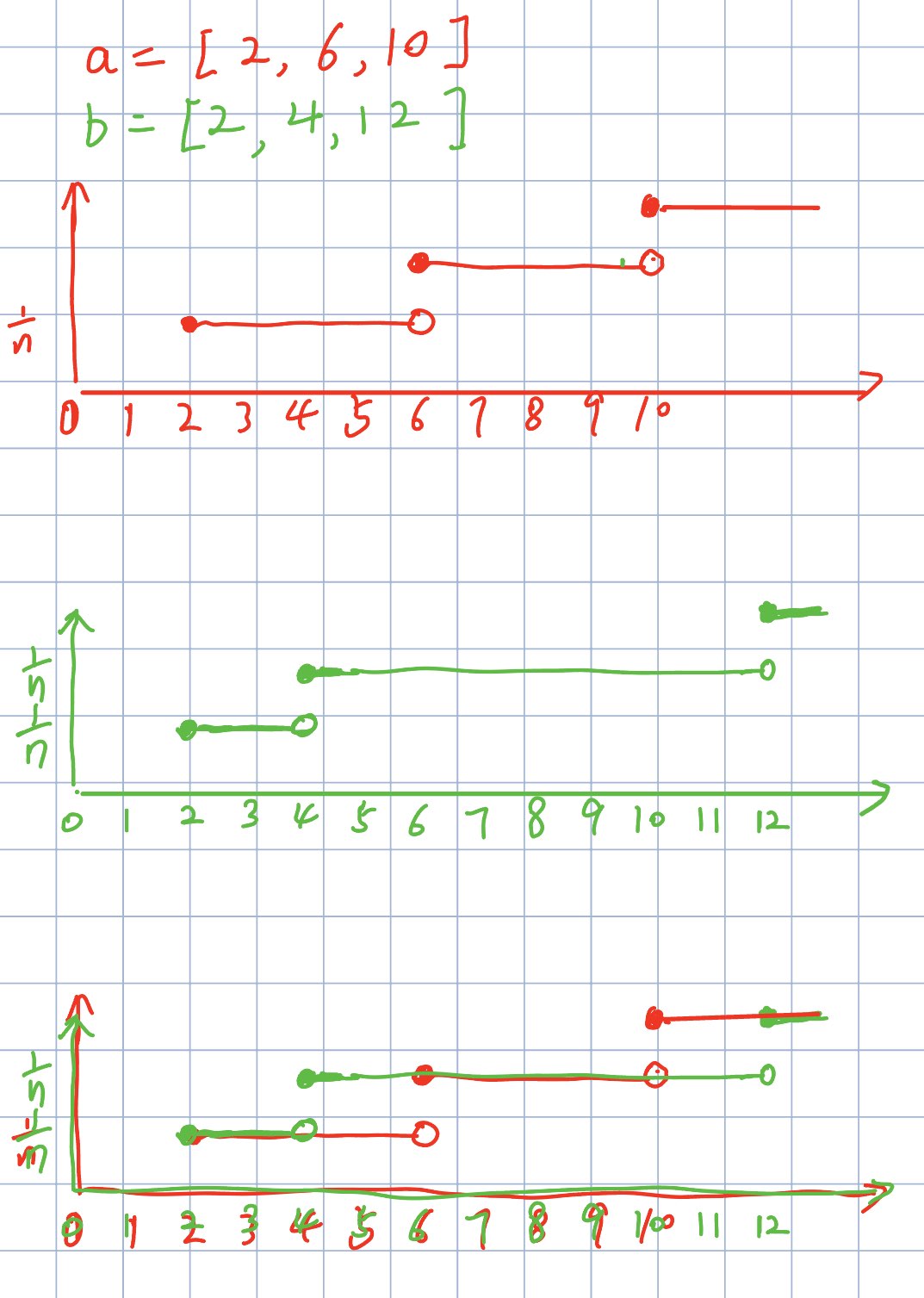emd_example

Find the cutoff point for CDF

all_values = [2, 2, 4, 6, 10, 12]

Merging the lists of u and v is equivalent to marking the positions of the values of two distribution on the coordinate axis, which is also the point of the Empircal CDF difference between the two distribution.
Get the CDF of each distribution
1. sort the two distribution in ascending order, u_values[u_sorter]=[2, 6, 10], v_values[v_sorter] = [2, 4, 12]
2. find the number of samples less than $x_i$, and than divide the size of distribution
  
  \[ \begin{equation} F_n(x_t) = \frac{\text{number of elements in the samples} \le x_t}{n} = \frac{1}{n}\sum_{i=1}^n I_{x_i \le x_t}, \end{equation} \]
u_cdf_indices = [1, 1, 1, 2, 3], v_cdf_indices= [1, 1, 2, 2, 2]

CDF = u_cdf_indices / u_values.size

number of elements less than $x_i$ = u_values[u_sorter].searchsorted(all_values[:-1], 'right'). Due to the discrete nature, scipy get the CDF of the cutoff points (CDF different places) through the above code (Actually, we can calculate the CDF value at any discrete coordinate, but it's unnecessary; we only need to compute it for the cutoff coordinates). For instance, for the 3rd cutoff element $x_i = 4$, it find the number of elements less than $x_i = 4$ in u_values[u_sorter], which is the $F_X(x_i=4) * size(u\_values)$.

Although the cutoff point coordinate can be repeated, the distance between the two repeated points is 0, so it does not affect the calculation of the distance.
Get the CDF value differences of two distribution as the probability 'mass' in $x$.

np.abs(u_cdf - v_cdf): the difference of empirical CDF values at the cutoff points, which is the probability 'mass' in $x$.
Get the distance to move from $u_i$ to $v_i$.

deltas = np.diff(all_values): the distance between two cutoff points, which is the distance to move from $u_i$ to $v_i$.
Sum the multiplication of the above two values in terms of $x$

For instance, when $4 \le x_i \lt 6$,

$F_X(4)$ = u_cdf($X \le x_i$) = u_cdf[2] = 1

$F_Y(4)$ = v_cdf($Y \le x_i$) = v_cdf[2] = 2$

delta[2] =all_values[3] - all_values[2] =6-4=2

According to Equation 7, the distance to move from $u_i$ to $v_i$ in $F(4)$ is $2*|1-2| = 2$.

Recommend for Corresponding Python code: Python 计算累积分布函数 CDF 并绘图_python cdf 函数-CSDN 博客

More Examples and Tests for other libraries

scipy use cases

from scipy.stats import wasserstein_distance

def wassersteindist(n):
    a = np.random.randn(n)
    b = np.random.randn(n)
    w = wasserstein_distance(a,b)
    return w

print(np.mean([wassersteindist(100) for r in range(1000)]))
print(np.mean([wassersteindist(1000) for r in range(1000)]))
print(np.mean([wassersteindist(10000) for r in range(1000)]))
# OUTPUT
# 0.17644314409413253
# 0.05818221578545196
# 0.018522773678086024

解读：np.random.randn 返回标准正态分布(mean=0, std=1, Gaussian distribution) 的采样, a, b 都是同一分布的采样点。对于同一分布采样点来说，样本量越大越接近其分布，而二者分布一样，因此二者的 wasserstein distance 随着样本量逐渐增大会趋近于 0。

Wasserstein 距离是一种用于衡量两个概率分布之间距离的方法，它考虑了分布之间的相似性和几何距离之间的关系。它有许多应用，例如生成对抗网络（GAN）中的损失函数和图像检索中的相似性度量。

Wasserstein 距离的定义基于最小化将一个分布转换为另一个分布所需的成本。成本可以是任意的，但通常是指将一个分布中的质量从一个位置移动到另一个位置所需的成本。这个成本可以表示为两个位置之间的距离和质量的乘积。

from scipy.stats import wasserstein_distance

a, b = [2,1,3,4], [4,1,2,4]
w = wasserstein_distance(a,b)
print(w)

Wasserstein-p distance

如果要计算 p-Wasserstein distance between two 1d distributions, 也就是以 p 范数为距离衡量的 wasserstein distance，那 scipy 的功能就不行了，可以采用以下 PythonOT/POT: POT : Python Optimal Transport 的库函数：ot.wasserstein_1d(u_values, v_values, u_weights=None, v_weights=None, p=1, require_sort=True), 直接指定 p 范数的值即可。

import ot
pos_p, pos_q = np.array([0, 5]), np.array([0, 1])
counts_p, counts_q = np.array([3/4, 1/4]), np.array([1/2, 1/2])
ot.backend = 'numpy'

ot.wasserstein_1d(pos_p, pos_q, u_weights=counts_p, v_weights=counts_q, p=2, require_sort=True)

Difference between implementations of scipy， POT，and pyemd

这里比较 scipy 和 POT 的 wasserstein 函数和 pyemd 等库实现的差异。

1	scipy.stats.wasserstein_distance(u_values, v_values, u_weights=None， v_weights=None)

在 scipy 中，u_values, v_values 参数是从分布中采样的每个样本位置 (samples drawed from distribution) ，因此无顺序可重复（实际上看函数源码可以看到对其进行排序，也可以说明其无顺序），u_weight, v_weight 对应权重，质量。scipy 这种其实对机器学习中矩阵（都是样本）的距离计算挺方便的。

pyemd.emd(first_histogram,
    second_histogram,
    distance_matrix,
    extra_mass_penalty=-1.0)

pyemd 中，first_histogram，second_histogram 是分布的频率向量（pre-computed frequency vector about the distribution 或者也可以说是频率向量，mass 重量，权重，对应 scipy 中的 u_weight, v_weight, 并通过 distance_matrix 指定距离矩阵 specifying distances between bins.

因此，scipy 与 pyemd 之间的差异在于参数顺序以及位置和距离

计算两个矩阵之间的距离：

from scipy.stats import wasserstein_distance
import numpy as np
a = np.array([[3,4], [6,1]])
b = np.array([[68,1], [921,4]])
len = a.size
wasserstein_distance(np.arange(len), np.arange(len), a.flatten(), b.flatten())

输出：

1	0.6438631790744466

import pyemd
import numpy as np

def dist_matrix(len):
    dist = np.empty((len, len))
    for i in range(len):
        for j in range(len):
            dist[i][j] = abs(i-j)
    return dist

a = np.array([[3,4], [6,1]])
b = np.array([[68,1], [921,4]])
freq = lambda x: x.flatten() / np.sum(x) # compute the normalized histogram、frequency of each element

pyemd.pyemd.emd(freq(a), freq(b), dist_matrix(a.size)) # cost of moving mass under L1 is constant

输出

1	OUTPUT: 0.643861793763

看得出来直接计算矩阵的距离的话，用 scipy 还是挺方便的，便于在机器学习中应用。

Applications in Machine Learning

Image Generation and Style Transfer, 在生成对抗网络 GAN 中，测量真实分布与生成分布之间的距离，来构成目标函数，训练 GAN，提高生成图片的质量
Domain Adaptation, 量化源域与目标域的概率分布差异，从而调整源域上训练的模型
Outlier Detection, 将正常分布与潜在的异常分布做对比，通过捕捉质量和位置的差异，来识别异常值
数据增强，在增强训练数据时，从尽可能接近原始数据分布的分布中进行采样来生成真实的合成值。

Delve into Wasserstein Distance, principles and implementation analysis

Delve into Wasserstein Distance, principles and implementation analysis

Wasserstein distance

Definitions

Two equavalent formulas

Three intuitive and typical examples

Python tools for implementation

scipy 1d Wasserstein distance

scipy.stats.wasserstein_distance sourcecode analysis

More Examples and Tests for other libraries

scipy use cases

Wasserstein-p distance

Difference between implementations of scipy， POT，and pyemd

Applications in Machine Learning

References and Recommends